 =
=  =
=
By the end of this chapter student should be able to:
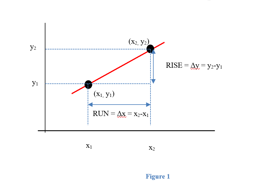
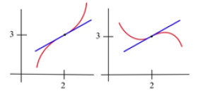
The slope of a line measures how fast a line rises or falls as we move from left to right along the line. It measures the rate of change of the y-coordinate with respect to changes in the x-coordinate. If the line represents the distance traveled over time, for example, then its slope represents the velocity. In Figure 1, you can remind yourself of how we calculate slope using two points on the line:
m = < slope from P to Q >= = =
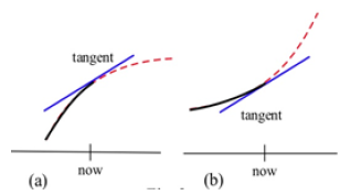
We would like to be able to get that same sort of information (how fast the curve rises or falls, velocity from distance) even if the graph is not a straight line. But what happens if we try to find the slope of a curve, as in Figure 2? We need two points in order to determine the slope of a line. How can we find a slope of a curve, at just one point?
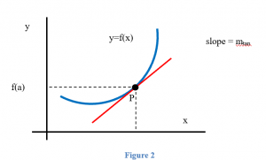
The answer, as suggested in Figure 2 is to find the slope of the tangent line to the curve at that point. Most of us have an intuitive idea of what a tangent line is. Unfortunately, “tangent line” is hard to define precisely.
Definition: A secant line is a line between two points on a curve.
Can’t-quite-do-it-yet Definition: A tangent line is a line at one point on a curve …. that does its best to be the curve at that point?
It turns out that the easiest way to define the tangent line is to define its slope.
The graph below is the graph of . We want to find the slope of the tangent line at the point (1, 2).
First, draw the secant line between (1, 2) and (2, −1) and compute its slope.
Now draw the secant line between (1, 2) and (1.5, 1) and compute its slope.
Compare the two lines you have drawn.
Which would be a better approximation of the tangent line to the curve at (1, 2)?
Now draw the secant line between (1, 2) and (1.3, 1.5) and compute its slope.
Is this line an even better approximation of the tangent line?
Now draw your best guess for the tangent line and measure its slope. Do you see a pattern in the slopes?
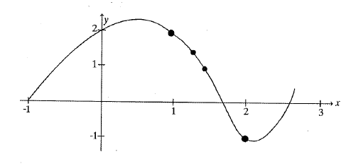
You should have noticed that as the interval got smaller and smaller, the secant line got closer to the tangent line and its slope got closer to the slope of the tangent line. That’s good news – we know how to find the slope of a secant line.
Example: Now let’s look at the problem of finding the slope of the line L (Figure 4) which is tangent to f(x) = x2 at the point (2,4).
We could estimate the slope of L from the graph, but we won’t. Instead, we will use the idea that secant lines over tiny intervals approximate the tangent line.
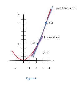
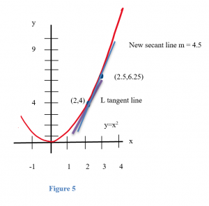
We can see that the line through (2,4) and (3,9) on the graph of f is an approximation of the slope of the tangent line, and we can calculate that slope exactly: m = ∆y/∆x = (9–4)/(3–2) = 5. But m = 5 is only an estimate of the slope of the tangent line and not a very good estimate. It’s too big. We can get a better estimate by picking a second point on the graph of f which is closer to (2,4) –– the point (2,4) is fixed and it must be one of the points we use. From Figure 5, we can see that the slope of the line through the points (2,4) and (2.5,6.25) is a better approximation of the slope of the tangent line at (2,4): m = ∆y/∆x = (6.25 – 4)/(2.5 – 2) = 2.25/.5 = 4.5 , a better estimate, but still an approximation. We can continue picking points closer and closer to (2,4) on the graph of f, and then calculating the slopes of the lines through each of these points and the point (2,4):
Points to the left of (2,4)
slope of line through
Points to the right of (2,4)
slope of line through
The only thing special about the x–values we picked is that they are numbers which are close, and very close, to x = 2. Someone else might have picked other nearby values for x. As the points we pick get closer and closer to the point (2,4) on the graph of y = x 2 , the slopes of the lines through the points and (2,4) are better approximations of the slope of the tangent line, and these slopes are getting closer and closer to 4.
We can bypass much of the calculating by not picking the points one at a time: let’s look at a general point near (2,4). Define x = 2 + h so h is the increment from 2 to x (Fig. 6). If h is small, then x = 2 + h is close to 2 and the point (2+h, f(2+h) ) = (2+h, (2+h)2 ) is close to (2,4). The slope m of the line through the points (2,4) and (2+h, (2+h)2 ) is a good approximation of the slope of the tangent line at the point (2,4):
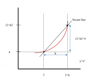
m= =
= =
= =
=  =
=  = .
= .
If h is very small, then m = 4 + h is a very good approximation to the slope of the tangent line, and m = 4 + h is very close to the value 4.
The value m = 4 + h is the slope of the secant line through the two points (2,4) and ( 2+h, (2+h) 2 ). As h gets smaller and smaller, this slope approaches the slope of the tangent line to the graph of f at (2,4).
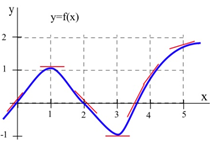
In some applications, we need to know where the graph of a function f(x) has horizontal tangent lines (slopes = 0). In Fig. 3, the slopes of the tangent lines to graph of y = f(x) are 0 when x = 2 or x ≈ 4.5 .
Example:At right is the graph of y = g(x). At what values of x does the graph of y = g(x) in Fig. 7 have horizontal tangent lines?
Solution:The tangent lines to the graph of g are horizontal (slope = 0) when x ≈ –1, 1, 2.5, and 5.
To know how rapidly something was changing at an instant in time the answer turns out to be to find the slope of a tangent line, which we approximate with the slope of a secant line. This idea is the key to defining the slope of a curve.
The derivative of a function f at a point (x, f(x)) is the instantaneous rate of change. The derivative is the slope of the tangent line to the graph of f at the point (x, f(x)). The derivative is the slope of the curve f(x) at the point (x, f(x)). A function is called differentiable at (x, f(x)) if its derivative exists at (x, f(x)).
Notation for the Derivative:
The derivative of y = f(x) with respect to x is written as:
(read aloud as “f prime of x”), or (“y prime”) or

(read aloud as “dee why dee ex”), or

 written in Roman letters instead of Greek letters.
Verb forms:
We find the derivative of a function,
or take the derivative of a function,
or differentiate a function.
notation to mean “find the derivative of f(x):”
Formal Algebraic Definition:
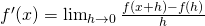
Practical Definition:
The derivative can be approximated by looking at an average rate of change, or the slope of a secant line, over a very tiny interval. The tinier the interval, the closer this is to the true instantaneous rate of change, slope of the tangent line, or slope of the curve.
Looking Ahead:
We will have methods for computing exact values of derivatives from formulas soon. If the function is given to you as a table or graph, you will still need to approximate this way.
This is the foundation for the rest of this chapter. It’s remarkable that such a simple idea (the slope of a tangent line) and such a simple definition (for the derivative f ‘ ) will lead to so many important ideas and applications.
We now know how to find (or at least approximate) the derivative of a function for any x-value; this means we can think of the derivative as a function, too. The inputs are the same x’s; the output is the value of the derivative at
Example: Fig. 8 is the graph of a function. We can use the information in the graph to fill in a table showing values of:
At various values of x, draw your best guess at the tangent line and measure its slope. You might have to extend your lines so you can read some points. In general, your estimate of the slope will be better if you choose points that are easy to read and far away from each other. Here are my estimates for a few values of x (parts of the tangent lines I used are shown):
f'(x) = the estimated SLOPE
of the tangent line to the curve
We can estimate the values of f’(x) at some non-integer values of x, too:
f’(.5) ≈ 0.5 and f’(1.3) ≈ –0.3.
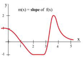
The values of f’(x) definitely depend on the values of x , and f’(x) is a function of x. We can use the results in the table to help sketch the graph of f’(x) in Fig. 9.
So far we have emphasized the derivative as the slope of the line tangent to a graph . That interpretation is very visual and useful when examining the graph of a function, and we will continue to use it. Derivatives, however, are used in a wide variety of fields and applications, and some of these fields use other interpretations. The following are a few interpretations of the derivative that are commonly used.
General
Rate of Change: f ‘(x) is the rate of change of the function at x. If the units for x are years and the units for f(x) are people, then the units for are  , a rate of change in population.
Graphical
Slope: f ‘(x) is the slope of the line tangent to the graph of f at the point ( x, f(x) )
Physical
Velocity: If f(x) is the position of an object at time x, then f ‘(x) is the velocity of the object at time x. If the units for x are hours and f(x) is distance measured in miles, then the units for f ‘(x) = are  ,miles per hour, which is a measure of velocity.
Acceleration: If f(x) is the velocity of an object at time x, then f ‘(x) is the acceleration of the object at time x. If the units are for x are hours and f(x) has the units , then the units for the acceleration f'(x)= are  =
=  , miles per hour per hour.
Business
Marginal Cost: If f(x) is the total cost of x objects, then f ‘(x) is the marginal cost, at a production level of x. This marginal cost is approximately the additional cost of making one more object once we have already made x objects. If the units for x are bicycles and the units for f(x) are dollars, then the units for f ‘(x) = are  , the cost per bicycle.
Marginal Profit: If f(x) is the total profit from producing and selling x objects, then f ‘(x) is the marginal profit, the profit to be made from producing and selling one more object. If the units for x are bicycles and the units for f(x) are dollars, then the units for f ‘(x) = are , dollars per bicycle, which is the profit per bicycle.
In business contexts, the word “marginal” usually means the derivative or rate of change of some quantity.
One of the strengths of calculus is that it provides a unity and economy of ideas among diverse applications. The vocabulary and problems may be different, but the ideas and even the notations of calculus are still useful.
Suppose you are producing and selling some item. The profit you make is the amount of money you take in minus what you have to pay to produce the items. Both of these quantities depend on how many you make and sell. (So we have functions here.) Here is a list of definitions for some of the terminology, together with their meaning in algebraic terms and in graphical terms.
Your cost is the money you have to spend to produce your items.
The Fixed Cost (FC) is the amount of money you have to spend regardless of how many items you produce. FC can include things like rent, purchase costs of machinery, and salaries for office staff. You have to pay the fixed costs even if you don’t produce anything.
The Total Variable Cost (TVC) for q items is the amount of money you spend to actually produce them. TVC includes things like the materials you use, the electricity to run the machinery, gasoline for your delivery vans, maybe the wages of your production workers. These costs will vary according to how many items you produce.
The Total Cost (TC) for q items is the total cost of producing them. It’s the sum of the fixed cost and the total variable cost for producing q items.
The Average Cost (AC) for q items is the total cost divided by q, or
 .
.
You can also talk about the average fixed cost,
 .
.
or the average variable cost,
 .
.
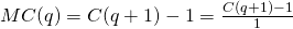
The Marginal Cost (MC) at q items is the cost of producing the next item. Really, it’s
MC(q) = TC(q + 1) – TC(q).
In many cases, though, it’s easier to approximate this difference using calculus (see Example below). And some sources define the marginal cost directly as the derivative,
In this course, we will use both of these definitions as if they were interchangeable.
Demand is the functional relationship between the price p and the quantity q that can be sold (that is demanded). Depending on your situation, you might think of p as a function of q, or of q as a function of p.
Your revenue is the amount of money you actually take in from selling your products. Revenue is price × quantity.
The Total Revenue (TR) for q items is the total amount of money you take in for selling q items.
The Average Revenue (AR) for q items is the total revenue divided by q, or
 .
.
The Marginal Revenue (MR) at q items is the cost of producing the next item,
MR(q) = TR(q + 1) – TR(q).
Just as with marginal cost, we will use both this definition and the derivative definition
Your profit is what’s left over from total revenue after costs have been subtracted.
The Profit (π) for q items is TR(q) – TC(q).
The average profit for q items is
 .
.
The marginal profit at q items is π(q + 1) – π(q), or π'(q)
Example: Why is it OK that are there two definitions for Marginal Cost (and Marginal Revenue, and Marginal Profit)?
We have been using slopes of secant lines over tiny intervals to approximate derivatives. In this example, we’ll turn that around – we’ll use the derivative to approximate the slope of the secant line.
Notice that the “cost of the next item” definition is actually the slope of a secant line, over an interval of 1 unit:
So this is approximately the same as the derivative of the cost function at q:
In practice, these two numbers are so close that there’s no practical reason to make a distinction. For our purposes, the marginal cost is the derivative is the cost of the next item.
Graphical Interpretations of the Basic Business Math Terms
Illustration/Example:
Here are the graphs of TR and TC for producing and selling a certain item. The horizontal axis is the number of items, in thousands. The vertical axis is the number of dollars, also in thousands.
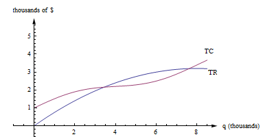
First, notice how to find the fixed cost and variable cost from the graph here. FC is the y-intercept of the TC graph. (FC = TC(0).) The graph of TVC would have the same shape as the graph of TC, shifted down. (TVC = TC – FC.)
We already know that we can find average rates of change by finding slopes of secant lines. AC, AR, MC, and MR are all rates of change, and we can find them with slopes, too.
AC(q) is the slope of a diagonal line, from (0, 0) to (q, TC(q)).
AR(q) is the slope of the line from (0, 0) to (q, TR(q)).
MC(q) = TC(q + 1) – TC(q), but that’s impossible to read on this graph. How could you distinguish between TC(4022) and TC(4023)? On this graph, that interval is too small to see, and our best guess at the secant line is actually the tangent line to the TC curve at that point. (This is the reason we want to have the derivative definition handy.)
MC(q) is the slope of the tangent line to the TC curve at (q, TC(q)).
In a similar way, MR(q) is the slope of the tangent line to the TR curve at (q, TR(q)).
Profit is the distance between the TR and TC curve. If you experiment with your clear plastic ruler, you’ll see that the biggest profit occurs exactly when the tangent lines to the TR and TC curves are parallel. This is the rule “profit is maximized when MR = MC.”
Example: You can estimate a tree’s age in years by multiplying its diameter (measured in inches) by its growth factor (a number that depends on the species). According to the Missouri Department of Conservation, the Growth factor for a cottonwood tree is 2.
Solution: a. The cottonwood tree should be about 6 × 2 = 12 years old.
b. The units of the growth factor are years per inch (because when we multiply the growth factor by inches, we get years).
c. Yes, the growth factor is a derivative. It has fractional units (years per inch), so it represents a rate. In this case, it’s the derivative of the function that gives the age of a tree as a function of its diameter. The function is linear, so the derivative in this case is the constant slope, 2 years per inch.
Example: The length of day (that is, daylight) in Seattle is a function of the day of the year. For example, on August 12 th , 2012, there were about 14 hours 24 minutes of daylight. In Seattle, August is the summer, approaching the autumnal equinox. The days are decreasing in length by about three minutes per day. So the derivative of this function is about −3 minutes per day. On January 15, 2012, which is wintertime in Seattle, there were about 8 hours 52 minutes of daylight, and the derivative was about (positive) 2 minutes per day; the length of the day was increasing by about 2 minutes a day.
In this section, we’ll get the derivative rules that will let us find formulas for derivatives when our function comes to us as a formula. This is a very algebraic section, and you should get lots of practice. When you tell someone you have studied calculus, this is the one skill they will expect you to have. There’s not a lot of deep meaning here – these are strictly algebraic rules.
These are the simplest rules – rules for the basic functions. We won’t prove these rules; we’ll just use them. But first, let’s look at a few so that we can see they make sense.
Example: Find the derivative of
Solution: This is a linear function, so its graph is its own tangent line! The slope of the tangent line, the derivative, is the slope of the line:
Rule: The derivative of a linear function is its slope
Example: Find the derivative of
Solution: Think about this one graphically, too. The graph of f(x) is a horizontal line. So its slope is zero.
Rule: The derivative of a constant is zero
Example: I will just tell you that the derivative of  is
is  . Now think about the function
  . What will its derivative be?
Solution: Think about what this change means to the graph of g – it’s now 4 times as tall as the graph of f. If we find the slope of a secant line, it will be  =
=  =
=  ; each slope will be 4 times the slope of the secant line on the f graph. This property will hold for the slopes of tangent lines, too:

Rule: Constants come along for the ride.
OK, enough of that. Here are the basic rules, all in one place.
Derivative Rules: Building Blocks
In what follows, f and g are differentiable functions of x.
| (a)Constant Multiple Rule: |  |
| (b)Sum (or Difference) Rule: |  or or  |
| (c) Power Rule: |  |
| Special cases: |  because because  |
 because because  | |
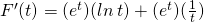
| (d) Exponential Functions: |  |
 | |
| (e)Natural Logarithm: |  |
The sum, difference, and constant multiple rule combined with the power rule allow us to easily find the derivative of any polynomial.

Solution:


No, you don’t have to show every single step. Do be careful when you’re first working with the rules, but pretty soon you’ll be able to just write down the derivative directly:
 =
=
The power rule works even if the power is negative or a fraction. In order to apply it, first translate all roots and one-overs into exponents:
![y=\sqrt[3]</p>
<p><strong>Example:</strong> Find the derivative of - \frac<t^> + 5e^](https://uw.pressbooks.pub/app/uploads/quicklatex/quicklatex.com-d1436340d46c6c9c4903a2a15ad65d47_l3.png)
Solution: First step – translate into exponents:
![y=\sqrt[3]</p>
<p> - \frac<t^> + 5e^=t^-4t^+ 5e^](https://uw.pressbooks.pub/app/uploads/quicklatex/quicklatex.com-c7d87fc19e5dfa80594472dc0bc958d3_l3.png)
Now you can take the derivative:
![\frac</p>
<p>(\sqrt[3] - \frac<t^> + 5e^)=\frac(\fract^-4t^+ 5e^)](https://uw.pressbooks.pub/app/uploads/quicklatex/quicklatex.com-f2021365c2a53906aaac5b7cb271d8e2_l3.png)

Be careful when finding the derivatives with negative exponents.
Example :
 hundred dollars.
(a) What is the cost for 100 items? 101 items? What is cost of the 101 st item?
, calculate f ‘(x) and evaluate f ‘ at x = 100.
How does f ‘(100) compare with the last answer in part (a)?
Solution:
(a)Put f(x) = =  hundred dollars, the cost for x items. Then f(100) = $1000 and f(101) = $1004.99, so it costs $4.99 for that 101 st item. Using this definition, the marginal cost is $4.99.
(b) f ‘(x) =  =
=  so f ‘(100) =
  =
=  hundred dollars = $5.00. Note how close these answers are! This shows (again) why it’s OK that we use both definitions for marginal cost.
The basic rules will let us tackle simple functions. But what happens if we need the derivative of a combination of these functions?
Solution: This function is not a simple sum or difference of polynomials. It’s a product of polynomials. We can simply multiply it out to find its derivative:


Solution: This function is not a simple sum or difference of polynomials. It’s a product of polynomials. We could simply multiply it out to find its derivative as before – who wants to volunteer? Nobody?
We’ll need a rule for finding the derivative of a product so we don’t have to multiply everything out.
Is the rule what we hope it is, that we can just take the derivatives of the factors and multiply them? Unfortunately, no – that won’t give the right answer.
Solution: We already worked out the derivative. It’s . What if we try differentiating the factors and multiplying them? We’d get  =
=  , which is totally different from the correct answer.
The rules for finding derivatives of products and quotients are a little complicated, but they save us the much more complicated algebra we might face if we were to try to multiply things out. They also let us deal with products where the factors are not polynomials. We can use these rules, together with the basic rules, to find derivatives of many complicated looking functions.
Derivative Rules: Product and Quotient Rules:
In what follows, f and g are differentiable functions of x.
The derivative of the first factor times the second left alone, plus the first left alone times the derivative of the second.
The product rule can extend to a product of several functions; the pattern continues – take the derivative of each factor in turn, multiplied by all the other factors left alone, and add them up.
The numerator of the result resembles the product rule, but there is a minus instead of a plus; the minus sign goes with the g’. The denominator is simply the square of the original denominator – no derivatives there.
Solution: This is a product, so we need to use the product rule. I like to put down empty parentheses to remind myself of the pattern; that way I don’t forget anything.
Then I fill in the parentheses – the first set gets the derivative of  , the second gets left alone, the third gets left alone, and the fourth gets the derivative of .
Notice that this was one we couldn’t have done by “multiplying out.”

Solution: This is a quotient, so we need to use the quotient rule. Again, I find it helpful to put down the empty parentheses as a template:
Then I fill in all the pieces:
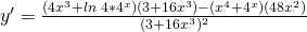
Now for goodness’ sakes don’t try to simplify that! Remember that “simple” depends on what you will do next; in this case, we were asked to find the derivative, and we’ve done that. Please STOP!
There is one more type of complicated function that we will want to know how to differentiate: composition. The Chain Rule will let us find the derivative of a composition. (This is the last derivative rule we will learn!)
Example: Find the derivative of .

Solution: This is not a simple polynomial, so we can’t use the basic building block rules yet. It is a product, so we could write it as and use the product rule. Or we could multiply it out and simply differentiate the resulting polynomial. I’ll do it the second way:


Solution: We could write it as a product with 20 factors and use the product rule, or we could multiply it out. But I don’t want to do that, do you?
We need an easier way, a rule that will handle a composition like this. The Chain Rule is a little complicated, but it saves us the much more complicated algebra of multiplying something like this out. It will also handle compositions where it wouldn’t be possible to “multiply it out.”
The Chain Rule is the most common place for students to make mistakes. Part of the reason is that the notation takes a little getting used to. And part of the reason is that students often forget to use it when they should. When should you use the Chain Rule? Almost every time you take a derivative.
Derivative Rules: Chain Rule
In what follows, f and g are differentiable functions with and
Notice that the du’s seem to cancel. This is one advantage of the Leibniz notation; it can remind you of how the chain rule chains together.
I recite the version in words each time I take a derivative, especially if the function is complicated.
Example: Find the derivative of .
Solution: This is the same one we did before by multiplying out. This time, let’s use the Chain Rule: The inside function is what appears inside the parentheses : . The outside function is the first thing we find as we come in from the outside – it’s the square function, something 2 . We want the derivative of the outside
(2 something) TIMES the derivative of what’s inside (which is ):

(By the way, if you multiply this out, you get the same answer we got before. Hurray! Algebra works!)
Solution: Now we have a way to handle this one. It’s the derivative of the outside TIMES the derivative of what’s inside.

 .
.
Solution: This isn’t a simple exponential function; it’s a composition. Typical calculator or computer syntax can help you see what the “inside” function is here. On a TI calculator, for example, when you push the key, it opens up parentheses: This tells you that the “inside” of the exponential function is the exponent. Here, the inside is the exponent . Now we can use the Chain Rule: We want the derivative of the outside TIMES the derivative of what’s inside. The outside is the “e to the” function, so its derivative is the same thing. The derivative of what’s inside is 2x. So
A function is called differentiable at a point if its derivative exists at that point.
We’ve been acting as if derivatives exist everywhere for every function. This is true for most of the functions that you will run into in this class. But there are some common places where the derivative doesn’t exist.
Remember that the derivative is the slope of the tangent line to the curve. That’s what to think about.
Where can a slope not exist? If the tangent line is vertical, the derivative will not exist.
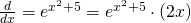
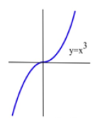
Example: This is the graph of f(x) = ![\sqrt[3]<x>](https://uw.pressbooks.pub/app/uploads/quicklatex/quicklatex.com-cade19ad1ffaa736832e7865abe1953a_l3.png) =
=  . Notice that the tangent line to this curve at x = 0 is vertical. So its slope does not exist, and so the derivative does not exist at x = 0.
Where can a tangent line not exist? If there is a corner in the graph, the derivative will not exist at that point because there is no well-defined tangent line (a teetering tangent, if you will.) Or if there is a jump in the graph, the tangent line will be different on either side and the derivative can’t exist.
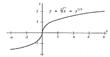
Example: This is the graph of the Greatest Integer Function, a basic step function. There is no single tangent line at x = 1; the tangent lines on either side are different. So the derivative does not exist at x = 1.
Graphically, a function is concave down if its graph is curved with the opening downward (Fig. 13a). Similarly, a function is concave up if its graph opens upward (Fig. 13b).
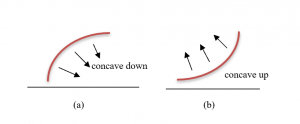
Example: An Epidemic: Suppose an epidemic has started, and you, as a member of congress, must decide whether the current methods are effectively fighting the spread of the disease or whether more drastic measures and more money are needed. In Fig. 14, f(x) is the number of people who have the disease at time x, and two different situations are shown. In both (a) and (b), the number of people with the disease, f(now), and the rate at which new people are getting sick, f ‘(now), are the same. The difference in the two situations is the concavity of f, and that difference in concavity might have a big effect on your decision.
In (a), f is concave down at “now”, the slopes are decreasing, and it looks as if it’s tailing off. We can say “f is increasing at a decreasing rate.” It appears that the current methods are starting to bring the epidemic under control.
In (b), f is concave up, the slopes are increasing, and it looks as if it will keep increasing faster and faster. It appears that the epidemic is still out of control.
The differences between the graphs come from whether the derivative is increasing or decreasing.
The derivative of a function f is a function that gives information about the slope of f. The derivative tells us if the original function is increasing or decreasing.
Because f ‘ is a function, we can take its derivative. This second derivative also gives us information about our original function f. The second derivative gives us a mathematical way to tell how the graph of a function is curved. The second derivative tells us if the original function is concave up or down.
Second Derivative
Let
The second derivative of f is the derivative of .
Using prime notation, this is or . You can read this aloud as “y double prime.”
Using Leibniz notation, the second derivative is written  or
or  . This is read aloud as “the second derivative of f.
If is positive on an interval, the graph of is concave up on that interval. We can say that f is increasing (or decreasing) at an increasing rate.
If is negative on an interval, the graph of is concave up on that interval. We can say that f is increasing (or decreasing) at a decreasing rate.
Example: Find for
Solution: First, we need to find the first derivative:
Then we take the derivative of that function:

Definition: An inflection point is a point on the graph of a function where the concavity of the function changes, from concave up to down or from concave down to up.
Example:Which of the labeled points in Fig. 15 are inflection points?
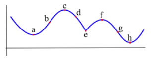
Solution: The concavity changes at points b and g. At points a and h, the graph is concave up on either side, so the concavity does not change. At points c and f, the graph is concave down on either side. And at point e, even though the graph looks strange there, the graph is concave down on both sides – the concavity does not change.
Inflection points happen when the concavity changes. Because we know the connection between the concavity of a function and the sign of its second derivative, we can use this to find inflection points.
Working Definition:An inflection point is a point on the graph where the second derivative changes sign.
In order for the second derivative to change signs, it must either be zero or be undefined. So to find the inflection points of a function we only need to check the points where f ”(x) is 0 or undefined.
Note that it is not enough for the second derivative to be zero or undefined. We still need to check that the sign of f’’ changes sign. The functions in the next example illustrate what can happen.
 (Fig. 16).
For which of these functions is the point (0,0) an inflection point?
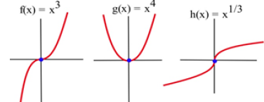
changes at (0,0), so (0,0) is an inflection point for f and h. The function is concave up everywhere so (0,0) is not an inflection point of g.
We can also compute the second derivatives and check the sign change.
If , then and . The only point at which f ”(x) = 0 or is undefined
(f ‘ is not differentiable) is at x = 0. If x < 0, then f ”(x) < 0 so f is concave down. If x >0 , then
f ”(x) > 0 so f is concave up. At x = 0 the concavity changes so the point (0,f(0)) = (0,0) is an inflection point of x3 .
If , then and . The only point at which or is undefined is at . If x < 0, then g ”(x) >0 so g is concave up. If x > 0 , then g ”(x) > 0 so g is also concave up. At x = 0 the concavity does not change so the point (0, g(0)) = (0,0) is not an inflection point of . Keep this example in mind!.
, then and . h” is not defined if x = 0, but h ”(negative number) > 0 and h ”(positive number) < 0 so h changes concavity at (0,0) and (0,0) is an inflection point of h.
Example: Sketch the graph of a function with f(2) = 3, f ‘(2) = 1, and an inflection point at (2,3) .
Solution: Two solutions are given in Fig. 17.
In theory and applications, we often want to maximize or minimize some quantity. An engineer may want to maximize the speed of a new computer or minimize the heat produced by an appliance. A manufacturer may want to maximize profits and market share or minimize waste. A student may want to maximize a grade in calculus or minimize the hours of study needed to earn a particular grade.
Without calculus, we only know how to find the optimum points in a few specific examples (for example, we know how to find the vertex of a parabola). But what if we need to optimize an unfamiliar function?
The best way we have without calculus is to examine the graph of the function, perhaps using technology. But our view depends on the viewing window we choose – we might miss something important. In addition, we’ll probably only get an approximation this way. (In some cases, that will be good enough.)
Calculus provides ways of drastically narrowing the number of points we need to examine to find the exact locations of maximums and minimums, while at the same time ensuring that we haven’t missed anything important.
Before we examine how calculus can help us find maximums and minimums, we need to define the concepts we will develop and use.
Definitions:
f has a local maximum at a if f(a) ≥ f(x) for all x near a
f has a local minimum at a if f(a) ≤ f(x) for all x near a
f has a local extreme at a if f(a) is a local maximum or minimum.
The plurals of these are maxima and minima. We often simply say “max” or “min;” it saves a lot of syllables.
Some books say “relative” instead of “local.”
The process of finding maxima or minima is called optimization.
A point is a local max (or min) if it is higher (lower) than all the nearby points. These points come from the shape of the graph.
Definitions:
f has a global maximum at a if f(a) ≥ f(x) for all x in the domain of f.
f has a global minimum at a if f(a) ≤ f(x) for all x in the domain of f.
f has a global extreme at a if f(a) is a global maximum or minimum.
Some books say “absolute” instead of “global”
A point is a global max (or min) if it is higher (lower) than every point on the graph. These points come from the shape of the graph and the window through which we view the graph.
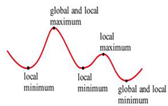
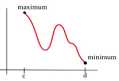
The local and global extremes of the function in Fig. 18 are labeled. You should notice that every global extreme is also a local extreme, but there are local extremes that are not global extremes.
If h(x) is the height of the earth above sea level at the location x, then the global maximum of h is h(summit of Mt. Everest) = 29,028 feet. The local maximum of h for the United States is h(summit of Mt. McKinley) = 20,320 feet. The local minimum of h for the United States is h(Death Valley) = – 282 feet.
Example: The table shows the annual calculus enrollments at a large university. Which years had local maximum or minimum calculus enrollments? What were the global maximum and minimum enrollments in calculus?
| Year | 2008 | 2009 | 2010 | 2011 | 2012 | 2013 | 2014 | 2015 | 2016 | 2017 | 2018 |
| Enrollment | 1257 | 1324 | 1378 | 1336 | 1389 | 1450 | 1523 | 1582 | 1567 | 1545 | 1571 |
Solution: There were local maxima in 2010 and 2015; the global maximum was 1582 students in 2015. There were local minima in 2011 and 2017; the global minimum was 1336 students in 2011. I choose not to think of 2008 as a local minimum or 2018 as a local maximum. However, some books would include the endpoints.
Finding Maxima and Minima of a Function
What must the tangent line look like at a local max or min? Look at these two graphs again – you’ll see that at all the extreme points, the tangent line is horizontal (so f’ = 0). There is one cusp in the blue graph – the tangent line if vertical there (so f’ is undefined).
That gives us the clue how to find extreme values.


Definition: A critical number for a function f is a value x = a in the domain of f where either f ’(a) = 0 or f ‘(a) is undefined.
Definition: A critical point for a function f is a point (a, f(a)) where a is a critical number of f.
Useful Fact: A local max or min of f can only occur at a critical point.

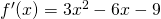
Example:Find the critical points of .
Solution: A critical number of f can occur only where f ‘(x) = 0 or where f’ does not exist.

so only at x = 1 and x = 3.
There are no places where f’ is undefined.
The critical numbers are x = 1 and x= 3. So the critical points are (1, 6) and (3, 2).
These are the only possible locations of local extremes of f. We haven’t discussed yet how to tell whether either of these points is actually a local extreme of f, or which kind it might be. But we can be certain that no other point is a local extreme.
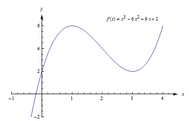
The graph of f (Fig. 19) shows that (1, f(1) ) = (1, 6) is a local maximum and (3, f(3) ) = (3, 2) is a local minimum. This function does not have a global maximum or minimum.
Example : Find all local extremes of .
Solution: is differentiable for all x, and . The only place where f ‘(x) = 0 is at x = 0, so the only candidate is the critical point (0,0). But if x > 0 then > 0 = f(0), so f(0) is not a local maximum. Similarly, if x < 0 then 0 = f(0) so f(0) is not a local minimum. The critical point (0,0) is the only candidate to be a local extreme of f, and this candidate did not turn out to be a local extreme of f. The function f(x) = x^3 does not have any local extremes. (Fig. 20)
Remember this example! It is not enough to find the critical points — we can only say that f might have a local extreme at the critical points.
Once we have found the critical points of f, we still have the problem of determining whether these points are maxima, minima or neither.
All of the graphs in Fig. 21 have a critical point at (2, 3). It is clear from the graphs that the point (2,3) is a local maximum in (a) and (d), (2,3) is a local minimum in (b) and (e), and (2,3) is not a local extreme in (c) and (f).
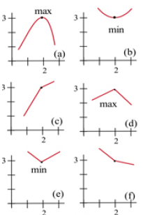
The critical numbers only give the possible locations of extremes, and some critical numbers are not the locations of extremes. The critical numbers are the candidates for the locations of maxima and minima.
f ‘ and Extreme Values of f
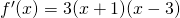
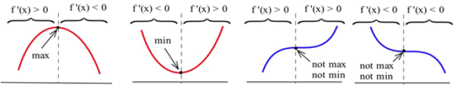
Four possible shapes of graphs are shown here – in each graph, the point marked by an arrow is a critical point, where f ‘(x) = 0. What happens to the derivative near the critical point?
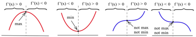
At a local max, such as in the graph on the left, the function increases on the left of the local max, then decreases on the right. The derivative is first positive, then negative at a local max. At a local min, the function decreases to the left and increases to the right, so the derivative is first negative, then positive. When there isn’t a local extreme, the function continues to increase (or decrease) right past the critical point – the derivative doesn’t change sign.
The First Derivative Test for Extremes:
Find the critical points of f.
For each critical number c, examine the sign of f’ to the left and to the right of c. What happens to the sign as you move from left to right?
If f ‘(x) changes from positive to negative at x = c, then f has a local maximum at (c, f(c)).
If f ‘(x) changes from negative to positive at x = c, then f has a local minimum at (c, f(c)).
If f ‘(x) does not change sign at x = c, then (c, f(c)) is neither a local max nor a local min.
Example:Find the critical points of and classify them as local max, local min, or neither..
Solution: We already found the critical points; they are (1, 6) and (3, 2).

Now we can use the first derivative test to classify each. Recall that . The factored form is easiest to work with here, so let’s use that.
(1, 6) – You could choose a number slightly less than 1 to plug into the formula for f’ – perhaps use x = 0, or
x = 0.9. Then you could examine its sign. But I don’t care about the numerical value, all I’m interested in is its sign. And for that, you don’t have to do any plugging in:
If x is a little less than 1, then x – 1 is negative, and x – 3 is negative. So f’ = 3(x – 1)(x – 3) will be pos(neg)(neg) = positive.
For x a little more than 1, you can evaluate f’ at a number more than 1 (but less than 3, you don’t want to go past the next critical point!) – perhaps x = 2. Or you can make a quick sign argument like what I did above. For x a little more than 1, f’ = 3(x – 1)(x – 3) will be pos(pos)(neg) = negative.
f’ changes from positive to negative, so there is a local max at (1, 6)
(3, 2) – f’ changes from negative to positive, so there is a local min at (3, 2).
This confirms what we saw before in the graph.

f ” and Extreme Values of f
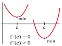
The concavity of a function can also help us determine whether a critical point is a maximum or minimum or neither. For example, if a point is at the bottom of a concave up function (Fig. 28), then the point is a minimum.
The Second Derivative Test for Extremes:
Find all critical points of f. For those critical points where f’(c) = 0, find f’’(c).
(b) If f ”(c) > 0 then f is concave up and has a local minimum at x = c.
(c) If f ”(c) = 0 then f may have a local maximum, a minimum or neither at x = c.
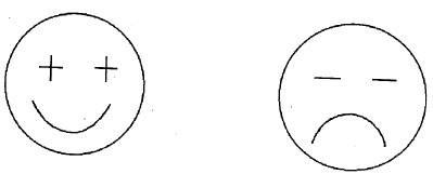
The cartoon faces can help you remember the Second Derivative Test.

Example: has critical numbers x = 1 and 4.
Use the Second Derivative Test for Extremes to determine whether f(1) and f(4) are maximums or minimums or neither.
Solution: We need to find the second derivative:
Then we just need to evaluate f ‘’ at each critical number:
x = 1: ; there is a local maximum at x = 1.
x = 4: ; there is a local minimum at x = 4.
Many students like the Second Derivative Test. The Second Derivative Test is often easier to use than the First Derivative Test. You only have to find the sign of one number for each critical number rather than two. And if your function is a polynomial, its second derivative will probably be a simpler function than the derivative.
But if you needed a product rule, quotient rule, or chain rule to find the first derivative, finding the second derivative can be a lot of work. And, even if the second derivative is easy, the Second Derivative Test doesn’t always give an answer. The First Derivative Test will always give you an answer.
Use whichever test you want to. But remember – you have to do some test to be sure that your critical point actually is a local max or min.
In applications, we often want to find the global extreme; knowing that a critical point is a local extreme is not enough.
For example, if we want to make the greatest profit, we want to make the absolutely greatest profit of all. How do we find global max and min? There are just a few additional things to think about.
Endpoint Extremes
The local extremes of a function occur at critical points – these are points in the function that we can find by thinking about the shape (and using the derivative to help us). But if we’re looking at a function on a closed interval, the endpoints could be extremes. These endpoint extremes are not related to the shape of the function; they have to do with the interval, the window through which we’re viewing the function.
In Fig. 26, it appears that there are three critical points – one local min, one local max, and one that is neither one. But the global max, the highest point of all, is at the left endpoint. The global min, the lowest point of all, is at the right endpoint.
How do we decide if endpoints are global max or min? It’s easier than you expected – simply plug in the endpoints, along with all the critical numbers, and compare y-values.

Example 3:Find the global max and min of for –2 ≤ x ≤ 6 .
Solution: = . We need to find critical points, and we need to check the endpoints.
(i) = 0 when x = –1 and x = 3.
(ii)f is a polynomial so f’ is defined everywhere.
(iii)The endpoints of the interval are x = –2 and x = 6.
Now we simply compare the values of f at these 4 values of x:
f(–2) = 3 , f(–1) = 10 , f(3) = –22 , and f(6) = 59.
The global minimum of f on [ –2, 6] is –22, when x = 3, and the global maximum of f on [ –2, 6] is 59, when x = 6.
If there’s only one critical point
If the function has only one critical point and it’s a local max (or min), then it must be the global max (or min). To see this, think about the geometry. Look at the graph on the left – there is a local max, and the graph goes down on either side of the critical point. Suppose there was some other point that was higher – then the graph would have to turn around. But that turning point would have shown up as another critical point. If there’s only one critical point, then the graph can never turn back around.
When in doubt, graph it and look.
If you are trying to find a global max or min on an open interval (or the whole real line), and there is more than one critical point, then you need to look at the graph to decide whether there is a global max or min. Be sure that all your critical points show in your graph, and that you go a little beyond – that will tell you what you want to know.
Example: Find the global max and min of .
Solution: We have previously found that (1, 6) is a local max and (3, 2) is a local min. This is not a closed interval, and there are two critical points, so we must turn to the graph of the function to find global max and min.
The graph of f (Fig. 28) shows that points to the left of x = 4 have y-values greater than 6, so (1, 6) is not a global max. Likewise, if x is negative, y is less than 2, so (3, 2) is not a global min. There are no endpoints, so we’ve exhausted all the possibilities. This function does not have a global maximum or minimum.

To find Global Extremes:
The only places where a function can have a global extreme are critical points or endpoints.
(a) If the function has only one critical point, and it’s a local extreme, then it is also the global extreme.
(b) If there are endpoints, find the global extremes by comparing y-values at all the critical points and at the endpoints.
(c) When in doubt, graph the function to be sure.
We have used derivatives to help find the maximums and minimums of some functions given by equations, but it is very unlikely that someone will simply hand you a function and ask you to find its extreme values. More typically, someone will describe a problem and ask your help in maximizing or minimizing something: “What is the largest volume package which the post office will take?”; “What is the quickest way to get from here to there?”; or “What is the least expensive way to accomplish some task?” In this section, we’ll discuss how to find these extreme values using calculus.
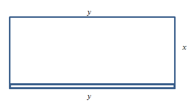
Example: The manager of a garden store wants to build a 600 square foot rectangular enclosure on the store’s parking lot in order to display some equipment. Three sides of the enclosure will be built of redwood fencing, at a cost of $7 per running foot. The fourth side will be built of cement blocks, at a cost of $14 per running foot. Find the dimensions of the least costly such enclosure.
The process of finding maxima or minima is called optimization. The function we’re optimizing is called the objective function. The objective function can be recognized by its proximity to “est” words (greatest, least, highest, farthest, most, …) Look at the garden store example; the cost function is the objective function.
In many cases, there are two (or more) variables in the problem. In the garden store example again, the length and width of the enclosure are both unknown. If there is an equation that relates the variables we can solve for one of them in terms of the others, and write the objective function as a function of just one variable. Equations that relate the variables in this way are called constraint equations. The constraint equations are always equations, so they will have equals signs. For the garden store, the fixed area relates the length and width of the enclosure. This will give us our constraint equation.
Once we have a function of just one variable, we can apply the calculus techniques we’ve just learned to find maxima or minima. Max-Min Story Problem Technique:
(a) Translate the English statement of the problem line by line into a picture (if that applies) and into math. This is often the hardest step!
(b) Identify the objective function. Look for “est” words.
(b1) If you seem to have two or more variables, find the constraint equation. Think about the English
meaning of the word “constraint,” and remember that the constraint equation will have an = sign.
(b2) Solve the constraint equation for one variable and substitute into the objective function. Now you have
an equation of one variable.
(c) Use calculus to find the optimum values. (Take derivative, find critical points, test. Don’t forget to check the endpoints!)
(d) Look back at the question to make sure you answered what was asked. Translate your number answer back into English.
Example: The manager of a garden store wants to build a 600 square foot rectangular enclosure on the store’s parking lot in order to display some equipment. Three sides of the enclosure will be built of redwood fencing, at a cost of $7 per running foot. The fourth side will be built of cement blocks, at a cost of $14 per running foot. Find the dimensions of the least costly such enclosure.
Solution: First, translate line by line into math and a picture:
Translation
The manager of a garden store wants to build a 600 square foot rectangular enclosure on the store’s parking lot in order to display some equipment.
Three sides of the enclosure will be built of redwood fencing, at a cost of $7 per running foot. The fourth side will be built of cement blocks, at a cost of $14 per running foot.
Find the dimensions of the least costly such enclosure.
Let x and y be the dimensions of the enclosure, with
y being the length of the side made of blocks.
Area = A = xy = 600
2x + y costs $7 per foot
y costs $14 per foot
Cost = C = 7(2x + y) + 14y = 14x + 21y
Find x and y so that C is minimized.
 , and then substitute into C:
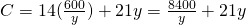
Now we have a function of just one variable, so we can whack it with calculus (find the critical points, etc.)
C’ is undefined for y = 0, and C’ = 0 when y = 20 or y = −20.
Of these three critical numbers, only y = 20 makes sense (is in the domain of the actual function) – remember that y is a length, so it can’t be negative. And y = 0 would mean there was no enclosure at all, so it couldn’t have an area of 600 square feet.
Test y = 20: (I chose the second derivative test)
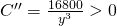
, so this is a local minimum.
Since this is the only critical point in the domain, this must be the global minimum. When y = 20, x = 30. The dimensions of the enclosure that minimize the cost are 20 feet × 30 feet.
You’ve probably heard before that “profit is maximized when marginal cost and marginal revenue are equal.” Now you can see why people say that! (Even though it’s not completely true.)
General Example: Suppose we want to maximize profit. Now we know what to do – find the profit function, find its critical points, test them, etc.
But remember that Profit = Revenue – Cost. So Profit’ = Revenue’ – Cost’. That is, the derivative of the profit function is MR – MC.
Now let’s find the critical points – those will be where Profit’ = 0 or is undefined.
Profit’ = 0 when MR – MC = 0, or where MR = MC.
That’s where the saying comes from! Here’s a more accurate way to express this:
Profit has critical points when Marginal Revenue and Marginal Cost are equal.
In all the cases we’ll see in this class, Profit will be very well behaved, and we won’t have to worry about looking for critical points where Profit’ is undefined. But remember that not all critical points are local max! The places where MR = MC could represent local max, local min, or neither one.
Example: A company sells q ribbon winders per year at $p per ribbon winder. The demand function for ribbon winders is given by:
The ribbon winders cost $30 apiece to manufacture, plus there are fixed costs of $9000 per year. Find the quantity where profit is maximized.
Solution: We want to maximize profit, but there isn’t a formula for profit showing … yet. So let’s make one. We can find a function for Revenue = pq using the demand function for p.

We can also find a function for Cost, using the variable cost of $30 per ribbon winder, plus the fixed cost:
Putting them together, we get a function for Profit:

Now we have two choices. We can find the critical points of Profit by taking the derivative of π(q) directly, or we can find MR and MC and set them equal. (Naturally, you’ll get the same answer either way.)
I’ll use MR = MC this time.
The only critical point is at q = 6750. Now we need to be sure this is a local max and not a local min. In this case, I’ll look to the graph of π(q) – it’s a downward opening parabola, so this must be a local max. And since it’s the only critical point, it must also be the global max.
Profit is maximized when they sell 6750 ribbon winders.
“Average cost is minimized when average cost = marginal cost” is another saying that isn’t quite true; in this case, the correct statement is:
Average Cost has critical points when Average Cost and Marginal Cost are equal.
Let’s look at a geometric argument here:

Remember that the average cost is the slope of the diagonal line, the line from the origin to the point on the total cost curve. If you move your clear plastic ruler around, you’ll see (and feel) that the slope of the diagonal line is smallest when the diagonal line just touches the cost curve – when the diagonal line is actually a tangent line – when the average cost is equal to the marginal cost.
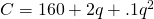
Example: The cost in dollars to produce q jars of gourmet salsa is given by . Find the quantity where the average cost is minimum.
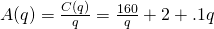 . We could find the critical points by finding , or by setting average cost to marginal cost; I’ll do the latter this time. . So I want to solve:
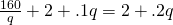

The critical point of average cost is when q = 40.
Notice that we still have to confirm that the critical point is a minimum. For this, we can use the first or second derivative test on .
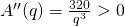
The second derivative is positive for all positive q, so that means this is a local min. Average cost is minimized when they produce 40 jars of salsa; at that quantity, the average cost is $10 per jar. (Mighty expensive salsa.)
We know that demand functions are decreasing, so when the price increases, the quantity demanded goes down. But what about revenue = price × quantity? Will revenue go down because the demand dropped so much? Or will revenue increase because demand didn’t drop very much?
Elasticity of demand is a measure of how demand reacts to price changes. It’s normalized – that means the particular prices and quantities don’t matter, so we can compare onions and cars. The formula for elasticity of demand involves a derivative, which is why we’re discussing it here .
Elasticity of Demand
Given a demand function that gives q in terms of p,
The elasticity of demand is
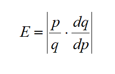
(Note that since demand is a decreasing function of p, the derivative is negative. That’s why we have the absolute values – so E will always be positive.)
If E > 1, we say demand is elastic. In this case, raising prices decreases revenue.
If E = 1, we say demand is unitary. E = 1 at critical points of the revenue function.
Example: A company sells q ribbon winders per year at $p per ribbon winder. The demand function for ribbon winders is given by:
Find the elasticity of demand when the price is $70 apiece. Will an increase in price lead to an increase in revenue?
Solution: First, we need to solve the demand equation so it gives q in terms of p, so that we can find :
so

Now compute elasticty.
The demand for products that people have to buy, such as onions, tends to be inelastic. Even if the price goes up, people still have to buy about the same amount of onions, and revenue will not go down. The demand for products that people can do without, or put off buying, such as cars, tends to be elastic. If the price goes up, people will just not buy cars right now, and revenue will drop.